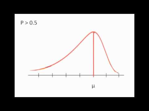
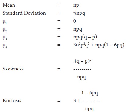
The expected value, or mean, of a binomial distribution, is calculated by multiplying the number of trials (n) by the probability of successes (p), or n x p. For example, the expected value of the You will begin with learning about the basic distribution types which include normal and binomial. STATISTICS FOR CONTROL GROUP A Mean: 4.5091 Std: 4.449 Var: 19.7939 Alpha: 1.0272 Beta: 0.2278. For instance, the binomial distribution tends to change into the normal distribution with mean and variance. The mean of the binomial distribution is n x p, the product of number of trials and the probability of success. The binomial distribution states the probability that a number of positive outcomes occurs given the expected percentage of positive outcomes and the total number of observations taken. Random variables fall into two broad categories: 1. 2017;6(1):1021. In this article I cover the method required to calculate statistical significance for non-binomial metrics such as average revenue per user, average order value, average sessions per user, average session duration, average pages per session, and others. Dirichlet Distribution; Poisson Distribution; Binomial Distribution and Random Walks; Runs; Statistical Power for One Sample Testing using Binomial Distribution; Sample Size Required Using the Poisson Distribution in Statistical Analyses. As an example, well walk through the assumptions for the binomial distribution. p: the event or success probability. of using appropriate distributions for statistical analysis. Select a different sub-topic. Am J Theoret Appl Stat. This is described by two constants, the mean m and the exponent k. 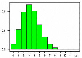The variance of the distribution is m2 (1) m + k ' the expected frequency In a binomial distribution the probabilities of interest are those of receiving a certain number of successes, say "k", in "n" independent trials each having only two possible outcomes and the Characteristics of Probability Distributions 2:05. To calculate the mean of a binomial distribution, We multiply N by P. In our case, this gives us a mean of seven, indicating we expect to sell seven showers on a typical day with 10 customers. Random variables A random variable is a variable whose value is subject to variations due to chance. If you satisfy the assumptions, you can use the distribution to model the process. Binomial Distribution Hypergeometric Distribution Poisson Distribution Continuous Distributions Binomial Experiments The Binomial Distribution The Mean and Standard Deviation Behavior of the Distribution Note that the binomial distribution is symmetric if p = 0:5, in which case the probability mass function simpli es to P(X = k) = nC k2 n. 1. This binomial distribution Excel guide will show you how to use the function, step by step. Analysts frequently use this probability distribution for quality control, survival analysis, and insurance analysis. 3. In this module you will be diving into the statistical side of Six Sigma. Enroll for Free. Statistical Analysis. Then the power of this test against alternative value p = 0.6 is given by P ( X 40 | n = 64, p = 0.6) = 0.3927. Each outcome has a fixed probability of occurring. most 3 chips fail in a random sample of 20. fGiven: Solution: ANSWER. For example, using the hsb2 data file, say we wish to test whether the proportion of females (female) differs significantly from 50%, i.e., from .5. In this article, we provide a general theory about the Poisson-Binomial distribution concerning its computation and applications, and Video unpacking question 12(a) from the NESA sample examination paper, which looks at the binomial distribution. Calculus. 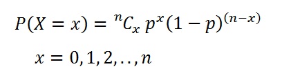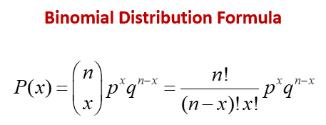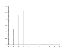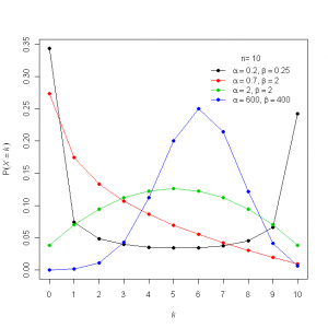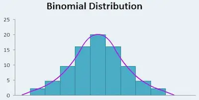The total probability variation of the control groups is decomposed into sample probability variation and probability variation between samples in control groups, the statistical analysis will be done to the data with binomial Binomial test. The binomial distribution has the following four assumptions: Each trial has one of two outcomes: This can be pass or fail, accept or reject, etc. fitted fairly well by a negative binomial distribution. This function reaches its maximum at p ^ = 1. If we observe X = 0 (failure) then the likelihood is L ( p; x) = 1 p, which reaches its maximum at p ^ = 0. Of course, it is somewhat silly for us to try to make formal inferences about on the basis of a single Bernoulli trial; usually, multiple trials are available. Here probability of getting head (p) is 0.5. In other words, events that can be categorized as either a successes or as a failure. Statistical Analysis Distributions: A distribution is simply a collection of data, or scores, on a variable. The negative binomial distribution looks like the Poisson distribution, except that it has a longer, fatter tail to the extent the variance exceeds the mean. P(x) = n1 x1 ( n x) 1p x(1 p)n x. 4. The statistical analysis of insect counts based on the negative binomial distribution. Bayes' Rule for Bayesian Inference. We discuss the use of the negative binomial (NB) distribution to evaluate performance instead of the commonly used Poisson Binomial distribution (henceforth NB, also known as over-dispersed Poisson) (Thall and Vail 1990). We can make a 'power curve' for this test by looking at a sequence of alternative values p.a between 0.5 and .75. The distribution is obtained by performing a number of Bernoulli trials. The first constructor takes one argument: the number of trials. In probability theory and statistics, the binomial distribution is the discrete probability distribution that gives only two possible results in an experiment, either Success or Failure. 1 or more accurately fr om the table in the Appendix, we can observe that the probability In the context of environmental statistics, the binomial distribution is sometimes used to model the proportion of times a chemical concentration exceeds a set standard in a given period of time (e.g., Gilbert, 1987, p.143). Use the binomial Binomial Distribution. A special case of binomial distribution. Explore statistical concepts in an interactive way. The resulting distribution looks similar to the binomial, with the skewness being positive but decreasing with l. Computing an interval probability using stats.binom. The outcomes of a binomial experiment fit a binomial probability distribution. Usually, these scores are arranged in order from smallest to largest and then they can be presented graphically. The BINOM.DIST Function [1] is categorized under Excel Statistical functions. For example, 1 - pbinom (39, 64, .6) [1] 0.392654. There is no intermediate result. The binomial distribution has two parameters, n and p. n: the number of trials. See calculation below for the mean and standard deviation of the number of heads (x) if we repeat it 100 times. interval_all_counts = range (21) probabilities = stats.binom.pmf (interval_all_counts, num_flips, prob_head) total_prob = the test run without a blowout. library (ggplot2) The binomial probability distribution models the discrete outcomes of dichotomous processes. The binomial distribution is used to determine the number of successes or failures for n number of attempts. This is the strength in our belief of without considering the evidence D. Our prior view on the probability of how fair the coin is. X ~ B ( n, p) Use the DCMP Data Analysis Tools to construct graphs, obtain summary statistics, find probabilities under the normal distribution, get confidence intervals, fit linear regression models, and more! The random variable X counts the number of successes obtained in the n independent trials. Usually, these scores are arranged in order from smallest to largest and then they can The binomial distribution is a discrete probability distribution that calculates the probability an event will occur a specific number of times in a set number of opportunities. This report presents simple statistical methods for analyzing binomial data, such as the number of failures in some number of demands. The binomial distribution is applied in binary outcomes events where the probability of success is equal to the probability of failure in The standard deviation is given by square root of np(1-p). When done without the replacement, the sampling may also be known as the You denote a binomial distribution as b(n,p). JABSTB: Statistical Design and Analysis of Experiments with R. Chapter 15 The Binomial Distribution. The new method of one-factor analysis of variance for medical statistical data with binomial distribution is studied in this paper. x is a vector of numbers.p is a vector of probabilities.n is number of observations.size is the number of trials.prob is the probability of success of each trial. A one sample binomial test allows us to test whether the proportion of successes on a two-level categorical dependent variable significantly differs from a hypothesized value.